Trajectory finding algorithm

The goal is to design an algorithm that could find in post treatment the trajectory of point with the equation of the ray that it emits during the experiment.

Summary of the equation

The problem will be easier to solve if the right mathematical formalism is given.

Ray

A ray can occur at any given time ($t_{r_p}$) with the equation of a line :

$$x_{r_p}(\lambda)= x_{g_{r_p}} + \lambda u_{r_p} , \ y_{r_p}(\lambda)= y_{g_{r_p}} + \lambda v_{r_p}$$

$x_{g_{r_p}} , y_{g_{r_p}}$ represent the generating point, $u_{r_p},v_{r_p}$ represent the direction of the ray

P.S. : It has been decided to use parametric formalism for line in order to streamline equation later…

Optimisation

The optimisation that should be undertaken, need to result to trajectory that minimize the difference with the true trajectory of the particle. In the same time, since we want to make this computation for a lot of different of ray in the continuous case. The optimisation problem should be as simple as possible.

Smallest distance

One can imagine to minimize the distance of the particle while going through every ray. It can be formulated easily like this :

$$(x_{m_{r_p}} , y_{m_{r_p}}){p \in [1,n]} = \argmin{(x_{m_{r_p}},y_{m_{r_p}}),p \in [1,n] } \sum_{p \in [1,n-1]} \left( x_{m_{r_p}}- x_{m_{r_{p+1}}} \right)^2 + \left( y_{m_{r_p}}- y_{m_{r_{p+1}}} \right)^2$$

$$\forall p \ \exists \lambda_p, \ x_{m_{r_p}}= x_{g_{r_p}} + \lambda_p u_{r_p}, \ y_{m_{r_p}}= y_{g_{r_p}} + \lambda_p v_{r_p}$$

One can apply a transformation in order to streamline the optimisation process

$$(\lambda_p){p \in [1,n]} = \ \argmin{(\lambda_p){p \in [1,n]} } \sum{p \in [1,n-1]} \left( x_{g_{r_p}} + \lambda_p u_{r_p}- x_{g_{r_{p+1}}} - \lambda_{p+1} u_{r_{p+1}} \right)^2 \ + \left( y_{g_{r_p}} + \lambda_p v_{r_p}- y_{g_{r_{p+1}}} - \lambda_{p+1} v_{r_{p+1}} \right)^2$$

We define a $P_p$ as :

$$P_p = \left( x_{g_{r_p}} + \lambda_p u_{r_p}- x_{g_{r_{p+1}}} - \lambda_{p+1} u_{r_{p+1}} \right)^2 \ + \left( y_{g_{r_p}} + \lambda_p v_{r_p}- y_{g_{r_{p+1}}} - \lambda_{p+1} v_{r_{p+1}} \right)^2$$

We can distribute the equation

$$P_p= \delta_{x_p}^2 + \lambda_p^2 u_{r_p}^2 + \lambda_{p+1}^2 u_{r_{p+1}}^2$$

$$+ \delta_{x_p} \lambda_p u_{r_p} - \delta_{x_p} \lambda_{p+1} u_{r_{p+1}} - \lambda_p u_{r_p} \lambda_{p+1} u_{r_{p+1}}$$

$$+ \delta_{y_p}^2 + \lambda_p^2 v_{r_p}^2 + \lambda_{p+1}^2 v_{r_{p+1}}^2$$

$$+ \delta_{y_p} \lambda_p v_{r_p} - \delta_{y_p} \lambda_{p+1} v_{r_{p+1}} - \lambda_p v_{r_p} \lambda_{p+1} v_{r_{p+1}}$$

With : $\delta_{x_p} = x_{g_{r_p}} - x_{g_{r_{p+1}}}, \ \delta_{y_p} = y_{g_{r_p}} - y_{g_{r_{p+1}}}$

After this step, different term should be grouped :

$$P_p =\left[ \lambda_p^2 \left( u_{r_p}^2 +v_{r_p}^2 \right) + \lambda_{p+1}^2 \left( u_{r_{p+1}}^2 + v_{r_{p+1}}^2 \right) - \lambda_p \lambda_{p+1} \left( v_{r_{p+1}} v_{r_p} + u_{r_{p+1}} u_{r_p}\right) \right]$$

$$+ \left[ \lambda_p \left( \delta_{x_p} u_{r_p} + \delta_{y_p} v_{r_p} \right) - \lambda_{p+1} \left( \delta_{x_p}u_{r_{p+1}} + \delta_{y_p} v_{r_{p+1}} \right) \right]$$

$$+ \left[ \delta_{x_p}^2 + \delta_{y_p}^2 \right]$$

The optimisation problem has been finaly formalised into the minimisation of a matrix second order polynome.

$$\Lambda_p = \begin{bmatrix} \lambda_p \ \lambda_{p+1} \end{bmatrix}^T ,$$

$$A_p =\begin{bmatrix} \left( u_{r_p}^2 +v_{r_p}^2 \right) & - \left( v_{r_{p+1}} v_{r_p} + u_{r_{p+1}} u_{r_p}\right) \- \left( v_{r_{p+1}} v_{r_p} + u_{r_{p+1}} u_{r_p}\right) & \left( u_{r_{p+1}}^2 + v_{r_{p+1}}^2 \right)\end{bmatrix}, $$

$$B_p = \begin{bmatrix} \left( \delta_{x_p} u_{r_p} + \delta_{y_p} v_{r_p} \right) \ - \left( \delta_{x_p}u_{r_{p+1}} + \delta_{y_p} v_{r_{p+1}} \right) \end{bmatrix},$$

$$C_p = \begin{bmatrix} \delta_{x_p}^2 + \delta_{y_p}^2 \end{bmatrix}$$

Finally $P_p$ can be summarised in the following :

$$P_p = \Lambda^T_p A_p \Lambda_p + B_p \Lambda_p + C_p$$

Finally one can group the $\left( P_p \right)_{p \in [1,n-1]}$ into an unique matrix problem :

$$\Lambda = \begin{bmatrix}
\lambda_1 \
\vdots \
\lambda_n
\end{bmatrix}^T$$

$$A = \begin{bmatrix} A^{(1)}{1,1} & A^{(1)}{1,2} \ A^{(1)}{2,1} & A^{(1)}{2,2} + A^{(2)}{1,1} & A^{(2)}{1,2}\ & A^{(2)}{2,1} & A^{(2)}{2,2}+ A^{(3)}{1,1} & \ddots \ & & \ddots & \ddots & A^{(p-1)}{1,2} \ & & & A^{(p-1)}{2,1} & A^{(p-1)}{2,2} \end{bmatrix}$$

$$B = \begin{bmatrix}B^{(1)}{1} \ B^{(1)}{2} + B^{(2)}{1} \ B^{(2)}{2} + B^{(3)}{1} \ \vdots \ B^{(p-1)}{2} \ \end{bmatrix}$$

$$C = \left[ \sum_{p=1}^{n-1} C_p \right]$$

By definition $A$ is semi definite positive (symetric). The solution of our problem is given by :
$$\Lambda = - \frac{1}{2} A^{-1}B$$

High order differentiation

Like the multiple ways existing to create continuous trajectory (B-spline, S pline ,etc…) It can be imagined to use these kind of higher order curve to approximate our trajectory.

Code and experimentation

We will show some code example and result of the above algorithm

Generation of situation

Concerning the simulation environment. It has been decided to simply follow a unique particle that move around randomly (at each timestep, change it speed and direction slightly) in a box. The particle randomly emit a ray.

Smallest distance

We gather the ray equation and apply the math above to return the list of lambda. Afterward we can determine the point guessed.

Result

We have compared the proposed method with the center average method used until know. A number of run has been made with different probability of ray emision.

Ray emited at each timestep :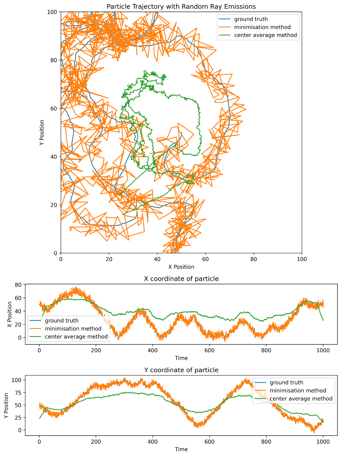

Ray emitted with a probability of 50% :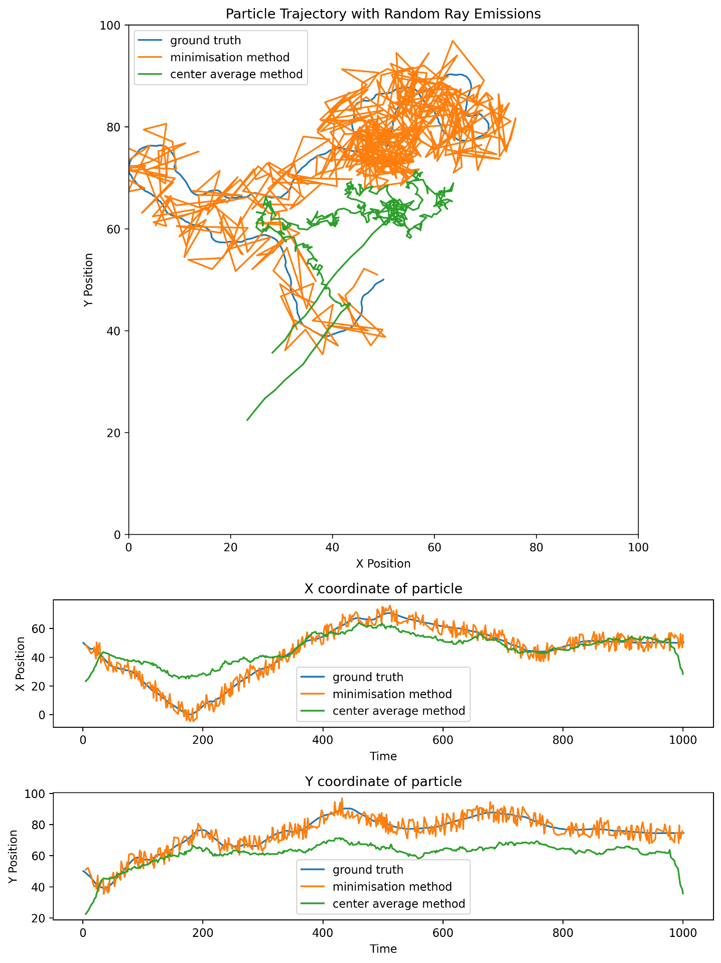

Ray emitted with a probability of 25% :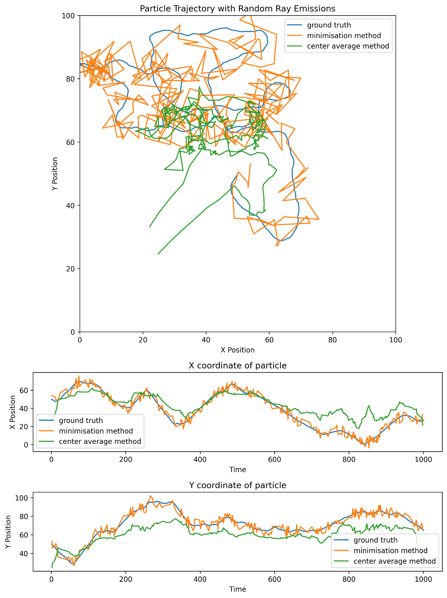

Ray emitted with a probability of 5% :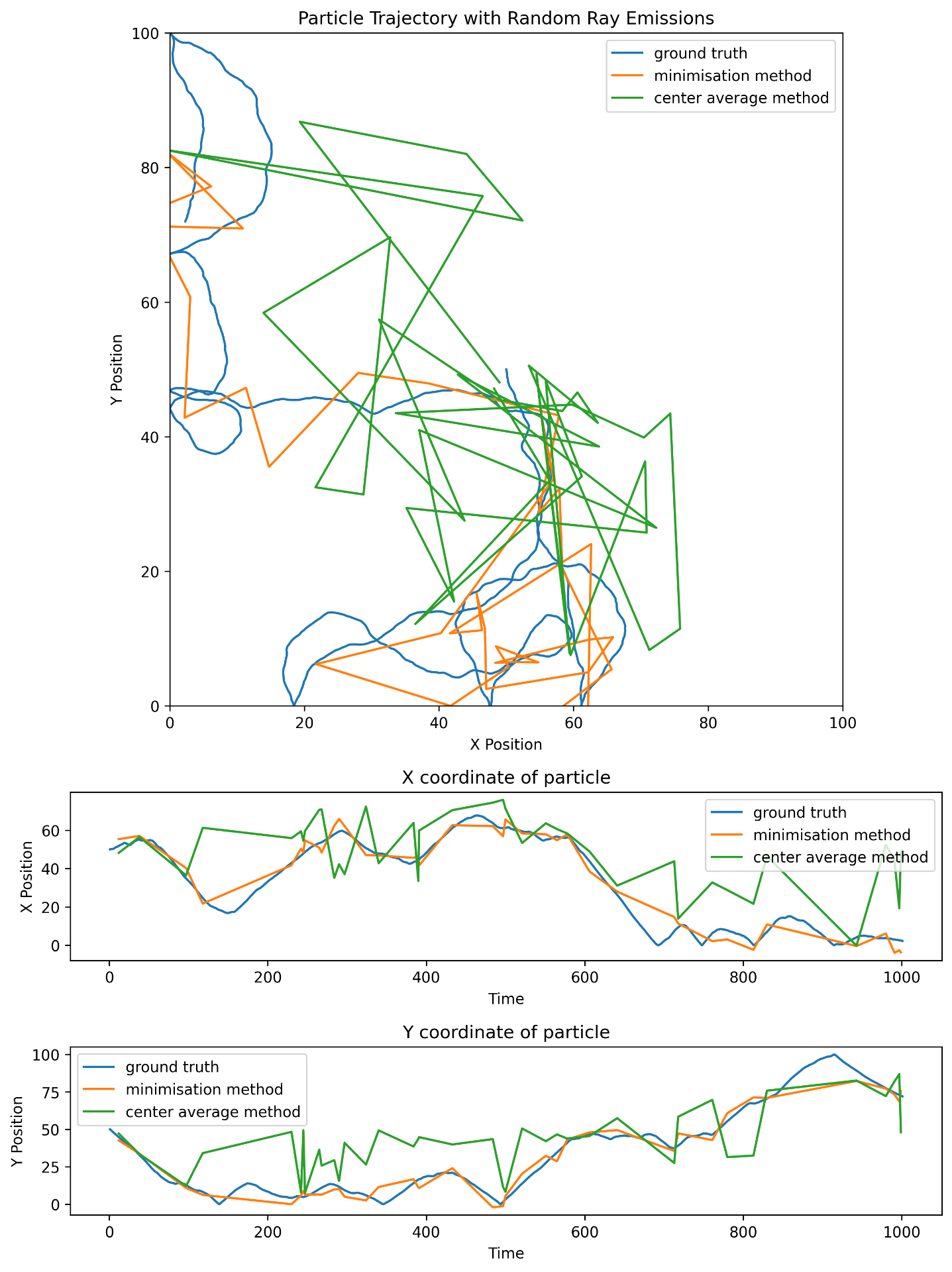

Conclusion

The raw result show that the method is working, however it is fairly noisy and further analysis should be made. In the same time, a method should be developped to take care of the probability distribution displacement over time.