May 2024
Meeting Report
Author: Eymeric Chauchat
Version: V1.0 (15 May 2024)
This is the first report - Next report
Introduction
This document summarizes the work on xL-Sindy from March through early May. Since this is the first report, I’ll include a global overview of the objectives.
Goal
Develop a complete framework using xL-Sindy to achieve optimal control for any given robot:
- Generalizability: xL-Sindy should remain general and free from prior knowledge constraints.
- Applicability: The framework should be adaptable for an ideal robot, Mujuco simulation, or real robot.
We can divide the framework into several core components:
- Generate Experiment Data
- Retrieve Dynamics Equations from Experiment Data
- Compute an optimal control policy based on the identified dynamics
- Implement the control policy on a real system
Currently, my focus is on the first two components. Specifically, I’ve worked on:
- Running ideal simulations
- Creating a force vector
- Formatting simulation data
- Retrieving dynamics equations
After detailing my work, I’ll present some preliminary results for the xL-Sindy Optimal Control framework.
Code Rebuild
Initially, I reviewed previous code related to this problem but found it challenging to understand the structure and methodology used in building xL-Sindy. As a result, I rewrote the code using a highly symbolic variable abstraction for Euler-Lagrange mechanics. Here’s an outline of the code structure:
Library Structure
The framework is structured as a Python library to organize each function:
Catalog_gen.py: Functions for creating the catalog of reference functions:Symbol_Matrix_g(Coord_number, t): Creates the symbolic matrix foundational to most functions dealing with dynamics.Concat_Func_var(f_cat, qk): Generates functions from a list of operators (e.g.,sin(),cos()) and a list of coordinates (q_0,q_1, …).Catalog_gen(f_cat, qk, degree, puissance=None): Creates polynomial combinations up to a specified degree, with an optional max power (puissance) for each element.Make_Solution_vec(exp, Catalog): Converts a symbolic expression into a solution vector.Make_Solution_exp(Solution, Catalog): Converts a solution vector into a symbolic expression.
Dynamics_modeling.py: Functions to run a Runge-Kutta 45 simulation on both the ideal and identified models.Euler_Lagrange.py: Functions to transform a symbolic Lagrangian expression into a time-dependent dynamic model.Euler_lagranged(expr, Smatrix, t, qi): Applies the Lagrangian transformation.Lagrangian_to_Acc_func(L, Symbol_matrix, t, Substitution, fluid_f=0): Converts the Lagrangian into an acceleration function.Catalog_to_experience_matrix(...): Converts the catalog of acceleration functions into a problem matrix, where columns represent catalog functions and rows are time points.
Optimization.py: Functions for performing linear regression on the problem matrix.Render.py: Functions to visualize results, such as rendering a pendulum’s motion over time.
Simulation Workflow
Steps to run a simulation using the library:
- Create the symbolic matrix for the experiment coordinates.
- Define the Lagrangian for the ideal system.
- Generate a time-varying force vector.
- Run a RK45 simulation to obtain position and speed over time.
- Create the function catalog.
- Form the experiment matrix.
- Apply a linear regression algorithm (typically LASSO for sparse discovery).
- Analyze the results.
Modifications to Original Code
I retained most of the algorithm’s functionality but didn’t include Yuan’s extension (for reasons explained later). I made several basic changes for generality:
- Automated simulation setup from the experiment’s Lagrangian.
- Altered function catalog creation to use polynomial combinations of basic components.
- Optimized the regression speed variable in LASSO.
Theoretical Modifications
Stochastic Excitation Vector
I discarded two of the three cases in the previous paper. First, the case with no external excitation was omitted because it heavily depends on system characteristics, and high dissipation forces can lead to insufficient data. I also excluded the case with prior knowledge, as it’s simply a restriction on input catalog functions.
The optimal force vector excites the system in a way that maximizes dynamics retrieval. The best approach was to interpolate a force function around randomly spaced points. This method has shown promising results for accurate dynamics retrieval.
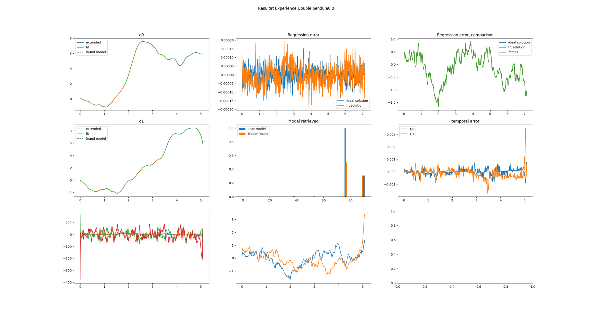
Viscous Forces
To handle viscous forces, I added them directly to the experiment matrix as they are non-conservative and cannot be included in the Lagrangian. This addition worked smoothly, improving convergence and allowing stronger excitations to enrich the learning data.
For example, the dynamics recovery achieved 89 basis functions with high accuracy, as shown in Figure 1.
Figure 1: Dynamics Retrieval of Double Pendulum
Results and Improvements
So far, I’ve focused on single and double pendulums, achieving:
- Dynamics recovery of damped systems with viscous forces.
- Faster dynamics recovery, requiring only 3 seconds of experimental data (compared to 5 seconds with 100 different initial conditions in past papers), achieving a precision of $4\text{e-}5$.
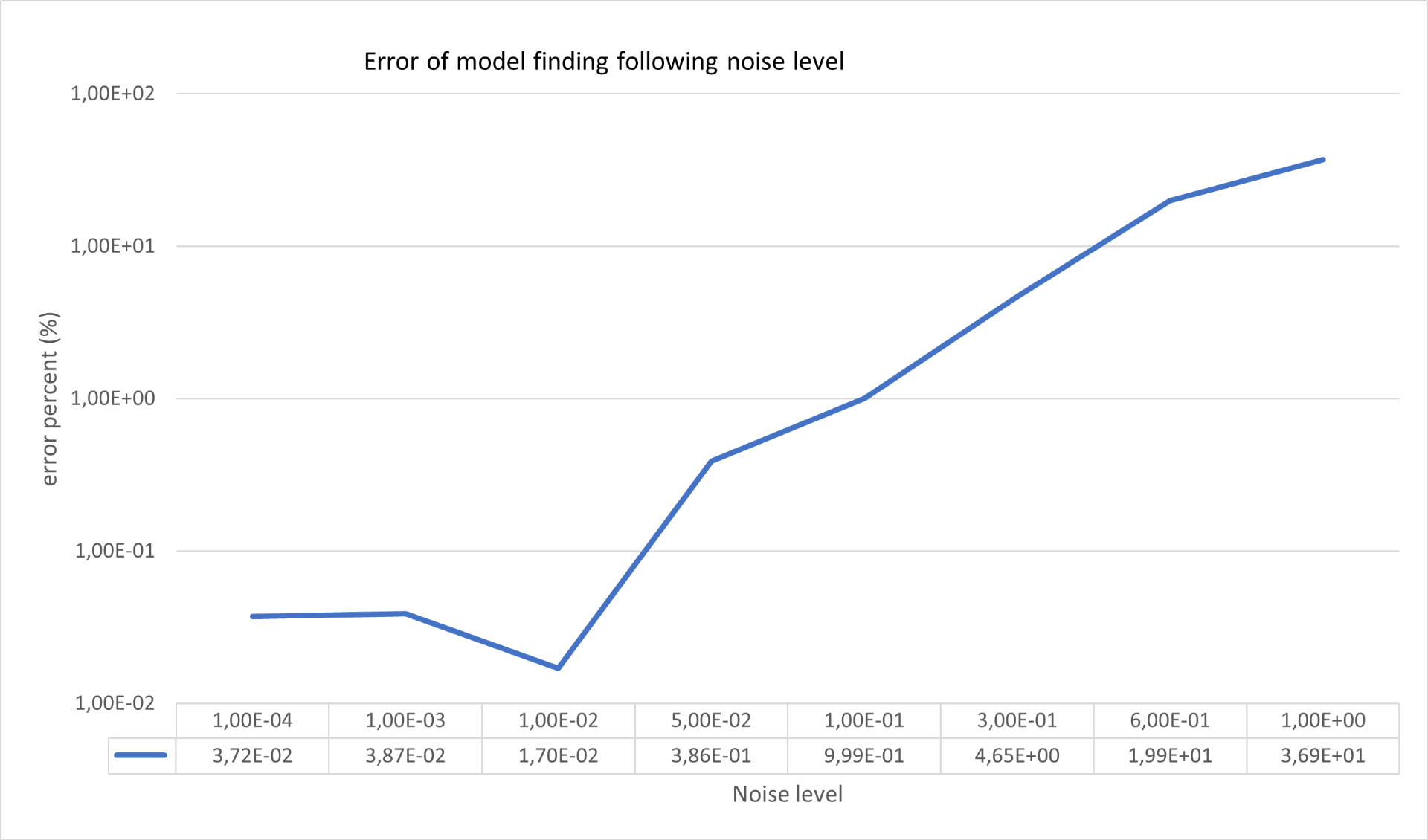
I also evaluated noise resilience (see Figure 2). With noise up to $1\text{e-}2$, the model consistently identified the correct functions. At noise levels of $1\text{e-}1$, a minor term was misidentified.
Figure 2: Noise Resilience of the Algorithm
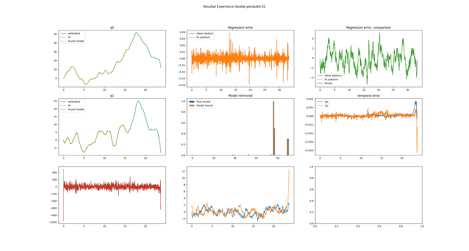
Example Experiment
Below is an example experiment (see Figure 3) conducted on a double pendulum with Gaussian noise of $1\text{e-}2$. The total experiment duration was 16 seconds with an oversampling factor of 25.
The ideal Lagrangian:
$$
0.004\dot{q_0}^2 + 0.004\dot{q_0}\dot{q_1}\sin(q_0)\sin(q_1) + 0.004\dot{q_0}\dot{q_1}\cos(q_0)\cos(q_1) + 0.002\dot{q_1}^2 + 0.3924\cos(q_0) + 0.1962 \cos(q_1)
$$
The retrieved Lagrangian:
$$
0.0039981\dot{q_0}^2 + 0.0039974\dot{q_0}\dot{q_1}\sin(q_0)\sin(q_1) + 0.0039985\dot{q_0}\dot{q_1}\cos(q_0)\cos(q_1) + 0.0019972\dot{q_1}^2 + 0.39214\cos(q_0) + 0.19611 \cos(q_1)
$$
Both viscous forces were also retrieved, achieving an overall precision of $2.4\text{e-}4$.
Figure 3: Example Experiment